Gradient Descent for Spectral Reconstruction

Using gradient descent to reconstruct UV/Vis absorption spectra of gold nanorods from a basis of simulated profiles

Gradient Descent for Spectral Reconstruction

UV/Vis spectroscopy can be used to learn about the size and shape of gold nanorods. Working with data form Gleason et al. (2024), I am trying to reconstruct the absorption spectra of gold nanorods using a basis of simulated absorption profiles.

I am using one of the simplest optimiztion methods to solve this problem: gradient descent.

Allthough quardatic methods like Gauss-Newton or Levenberg-Marquardt are more efficient, gradient descent is a good starting point to understand the problem and the solution space.

Problem to Solve

We want to solve the following non-negative least squares problem:

min ||A - P @ N||² subject to N ≥ 0

Where

• \(A\): Observed spectrum
• \(P\): Basis matrix of nanorod absorption profiles (K, IxJ)
  
• \(N\): Reconstruction coefficients (IxJ), to be solved

Basis functions

We have a couple of basis functions stored as JAX¹ arrays:

Shapes:
A shape: (167,)
P shape: (167, 10747)
Number of profiles: 10747
Number of wavelengths: 167

The number of basis functions exeeds the number of data points in the observed spectrum. This means that the problem is underdetermined, and we need to impose some constraints on the solution. In this case, we will use non-negativity constraints, which is common in spectral reconstruction problems.

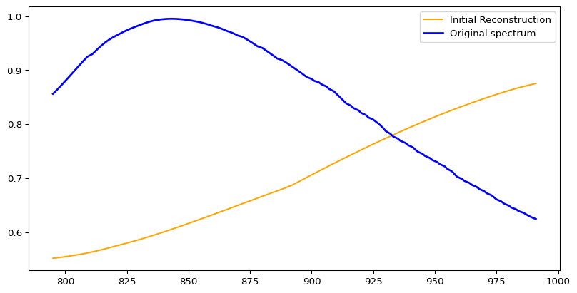
Initial Reconstruction

Initializing the weights uniformly gives us a profile to start with.

Gradient descent updates the coefficients iteratively to minimize the residuals between the observed spectrum and the reconstructed spectrum. It uses the gradient of the residuals to adjust the coefficients in the direction that reduces the residuals.

Reconstruction

After tuning the learning rate, the algorihtm converges:

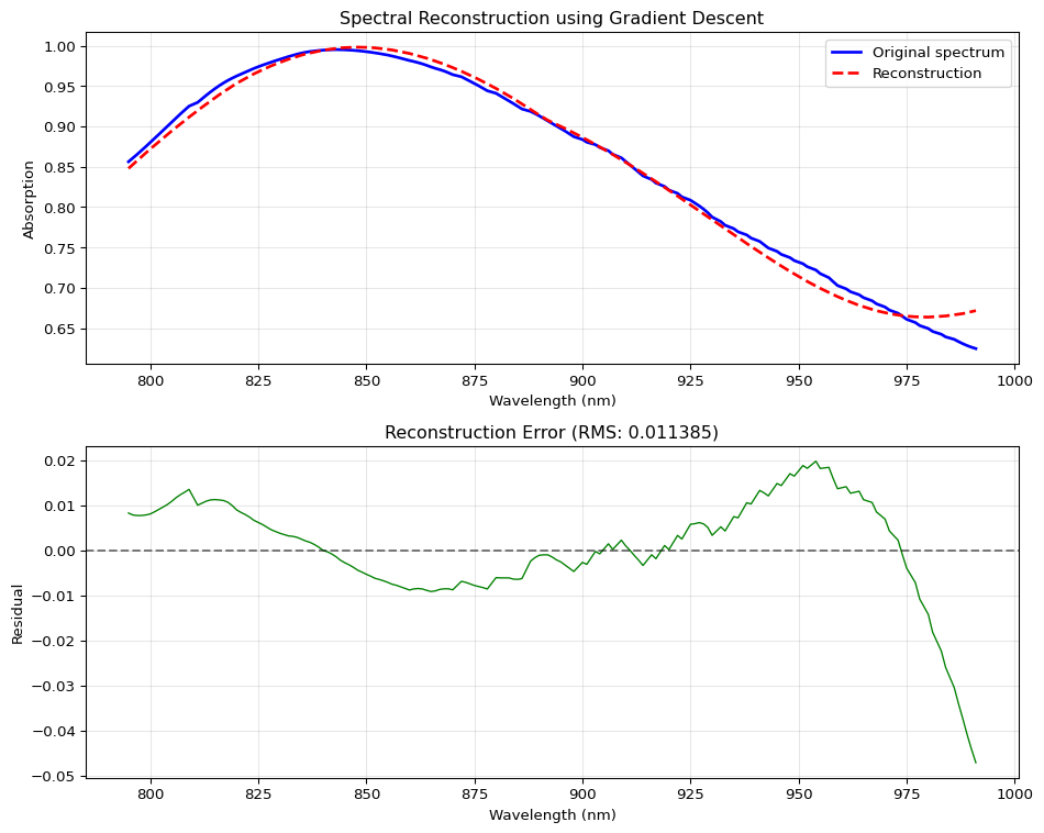
There are a couple of issues that I will address later

• Overshooting and undershooting behavoir
• How does solution depend on inital weights?

Overall the fit is not bad.

Solution Distribution Analysis

This is the distribution of the weights:

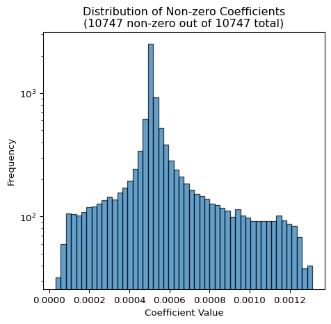
It is hard to interpret the distribution, as the coefficients make up a 2-dimensional vector. Interestingly, there is just one peak while later on we will see two peaks in the 2D distribution.

Population Heatmaps

In order to visualize the distribution of the coefficients, we can create a 2D heatmap:

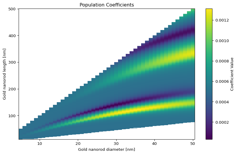
The are two peaks in the distribution. The contour lines of these peaks have banana shapes. This suggests that the length and diameter are correlated. This is typical for cristal stuctures, in which \(l/d\) is a constant. I will explore this in a future post.

Open questions:

• How to interpret the banana shape?
• Are the two peaks real?
• How unique is the decomposition?

Gleason, Samuel P., Jakob C. Dahl, Mahmoud Elzouka, Xingzhi Wang, Dana O. Byrne, Hannah Cho, Mumtaz Gababa, et al. 2024. “Automated Gold Nanorod Spectral Morphology Analysis Pipeline.” ACS Nano 18 (51): 34646–55. https://doi.org/10.1021/acsnano.4c09753.

Footnotes

1. JAX is a Python library for machine learning research that provides composable transformations of Python+NumPy programs: differentiation, vectorization, JIT compilation, and more. See jax.readthedocs.io for details.