Exploring Banana Shape Particle Distribution
spectral decomposition, particle distribution, naono rods
Exploring Banana Shape Particle Distribution
Sjoerd de Haan 2025-08-06
Original data
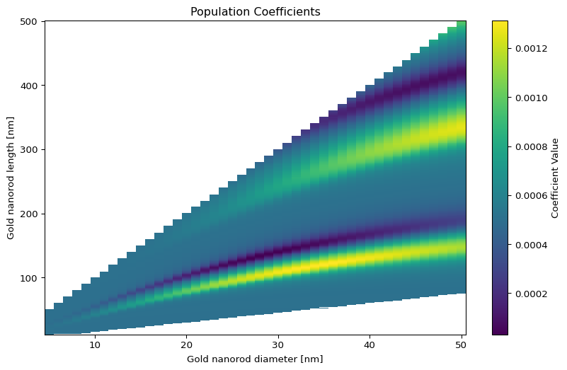
The first spectral decomposition I did showed banana shapes in the distribution of gold nanorods. Here I explore the banana shape and a possible relation to growth kinetics of gold crystals.
2D coefficients shape: (10747,)
Length range: 12.0 - 500.0 nm
Diameter range: 5.0 - 50.0 nm
Text(0.5, 1.0, 'Population Coefficients')- Population coefficients with banana-shaped contour lines
Contour lines
Let’s visualize those imagined contour lines:
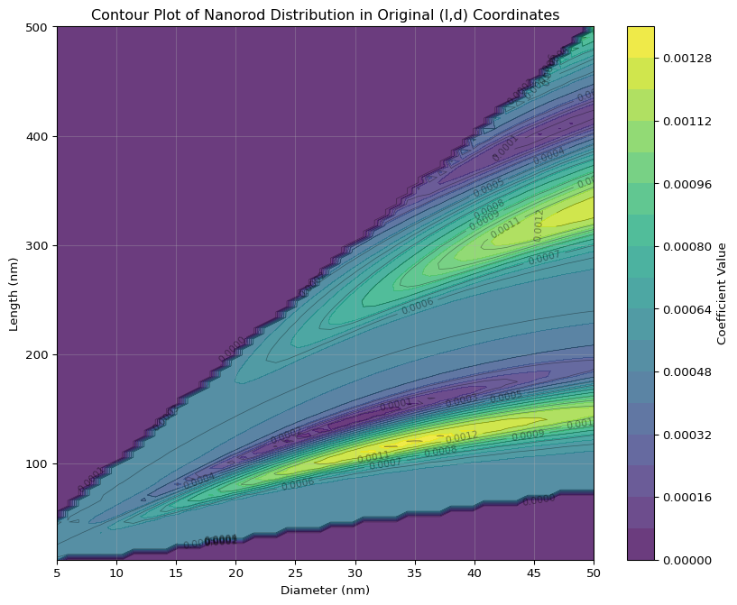
Indeed there is curvature visible in the contours.
Hypothesis
If the particle growth is constrained by crystal growth kinetics, we might expect the banana shape to be related to the aspect ratio of the particles. In this case we can
If aspect ration is fixed, then only diameter can vary. This not realistic. We expect variation in aspect ratio. This variation may be be independent of diameter, in which case the distribution factorizes into the product of the two marginals:
\[ p(d, l/d) = p(u, v) = p(d) \cdot p(l/d) \]
Coordinate Transformation
Gold crystals prefer to grow in certain directions. This can constrain the aspect ratios of nanoparticles.
To see if this is the case, we are going to transform to a new coordinate system from \((l, d)\) to \((u, v)\) where:
\[ \begin{align} u &= d \\ v &= \frac{l}{d} \end{align} \]
This is equivalently written as: \[ \begin{pmatrix} u \\ v \end{pmatrix} = \begin{pmatrix} d \\ l/d \end{pmatrix} \]
The inverse transformation is: \[ \begin{align} d &= u \\ l &= v \cdot u \end{align} \]
Jacobian and Density Compensation
When transforming probability densities, we need to account for the change in volume elements. If \(p_{ld}(l, d)\) is the probability density in the original coordinates and \(p_{uv}(u, v)\) is the density in the new coordinates, they are related by:
\[ p_{uv}(u, v) = p_{ld}(l, d) \left| \det \mathbf{J} \right| \]
where \(\mathbf{J}\) is the Jacobian matrix of the transformation from \((u, v)\) to \((l, d)\):
\[ \mathbf{J} = \frac{\partial(l, d)}{\partial(u, v)} = \begin{pmatrix} \frac{\partial l}{\partial u} & \frac{\partial l}{\partial v} \\ \frac{\partial d}{\partial u} & \frac{\partial d}{\partial v} \end{pmatrix} \]
Computing the partial derivatives: - \(\frac{\partial l}{\partial u} = \frac{\partial (v \cdot u)}{\partial u} = v\) - \(\frac{\partial l}{\partial v} = \frac{\partial (v \cdot u)}{\partial v} = u\) - \(\frac{\partial d}{\partial u} = \frac{\partial u}{\partial u} = 1\) - \(\frac{\partial d}{\partial v} = \frac{\partial u}{\partial v} = 0\)
Therefore: \[ \mathbf{J} = \begin{pmatrix} v & u \\ 1 & 0 \end{pmatrix} \]
The determinant is: \[ \det \mathbf{J} = v \cdot 0 - u \cdot 1 = -u = -d \]
Since we need the absolute value: \[ \left| \det \mathbf{J} \right| = |d| = d \]
Density Transformation Formula
Thus, the density compensation factor is \(d\), and the transformed density is:
\[ p_{uv}(u, v) = d \cdot p_{ld}(l, d) = u \cdot p_{ld}(v \cdot u, u) \]
This means that when we transform our coefficients from \((l, d)\) coordinates to \((d, l/d)\) coordinates, we need to multiply by the diameter \(d\) to preserve the total probability mass.
Implementing the Coordinate Transformation
The implementation is straightforward, thanks to xarray:
coeffs_compensated = coeffs_ds * coeffs_ds.diameter

# Create aspect ratio coordinate
aspect_ratio = coeffs.length / coeffs.diameter

# Add aspect ratio as a new coordinate
coeffs_with_ar = coeffs_compensated.assign_coords(aspect_ratio=aspect_ratio)

# Reset the current MultiIndex and create a new one with (diameter, aspect_ratio)
coeffs_transformed = coeffs_with_ar.reset_index('size_combo').set_index(size_combo=['diameter', 'aspect_ratio'])
Statistics
Here are the statistics of the old and new datasets:
Original index: (length, diameter)
New index: (diameter, aspect_ratio)
Number of data points: 10747

Unique diameters: 46
Unique aspect ratios: 6578
Actual data points: 10747
Scatter Plot Visualization
Now we have an irregular grid, we cannot use the heat map.
We can visualize the distribution in the new coordinate system using a scatter plot, where the color represents the coefficient values. This will help us see how the coefficients are distributed in the \((d, l/d)\) space.
![]()
This looks good! I see less curvature.
Interpolation to Regular Grid
To get a better image, I interpolate the data on a regular lattice, using scipy.interpolate.griddata. This will allow us to create a smooth surface that represents the distribution of coefficients in the \((d, l/d)\) space.
Regular grid shape: (100, 50)
Diameter grid: 50 points from 5.0 to 50.0 nm
Aspect ratio grid: 100 points from 1.51 to 10.00
Linear Interpolation
Linear interpolation creates a piecewise linear surface by:
- Triangulating the scattered points using Delaunay triangulation
- Within each triangle, fitting a plane through the three vertices
- Points outside the convex hull of the data get fill_value (0)
The “blocky” artifacts come from the patches meeting at triangle boundaries. Clipping removes negative values that physically don’t make sense for coefficient values.

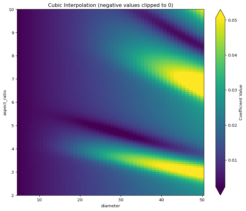
Cubic Interpolation
Cubic interpolation uses CloughTocher2DInterpolator which:
- Creates a triangulation with cubic polynomials
- Ensures C1 continuity (smooth first derivatives) across triangle boundaries
- Can produce oscillations and negative values due to polynomial overshoot
The “blocky” artifacts come from the cubic polynomial patches meeting at triangle boundaries. Clipping removes negative values that physically don’t make sense for coefficient values.
Contour Plot of Cubic Interpolation
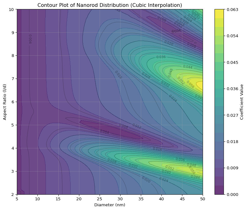
Observations
- There are two peaks in the distribution, perhaps even a third
- Diameter of nano rods exceeds 50 nm
- Next to the peaks there is a large valley
- There is less curvature to be seen compared to the original (l,d) coordinates
- The “banana” curvature is largely removed in the (d, l/d) coordinate system
- In the new coordinate, contours look elliptical near the peaks
Discussion
The banana shape likely arises from a coupling between length end diameter growth rated. This may come from crystal facets with different growth kinetics due to crystal structure and surfactant binding affinities.
The bi-modal distribution is consistent with several growth scenarios, including twinning, aggregative growth, or competing crystal structures.