Nano Particle Synthesis with Machine Learning
Can small machine learning experiments coupled with UV/Vis give insight into the synthesis of nanoparticles?
The paper that I read last week shows that it can!
Synthesis of Gold nanoparticles for Machine Learning
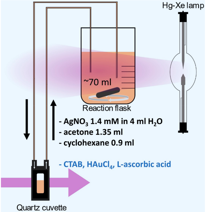
The authors of “Machine Learning Analysis of Reaction Parameters in UV-Mediated Synthesis of Gold Nanoparticles” Guda et al. (2023) employed a UV-mediated synthesis approach where gold nanoparticles were produced by mixing a gold precursor (HAuCl₄·4H₂O), a surfactant (hexadecyltrimethylammonium bromide or CTAB), a reducing agent (L-ascorbic acid), AgNO₃, acetone, and cyclohexane in a quartz vessel. The mixture was irradiated with UV light from a mercury-xenon lamp (386 W) for 60 minutes at a distance of 25 cm.
In this study, the authors systematically varied 3 of the syntisis parameters; the concentrations of
- gold precursor
- reducing agents
- surfactant
With a improved Latin hypercube sampling, they explored 30 different reaction conditions.
Meanwhile they monitored the reaction progress in real-time using in situ UV-vis spectroscopy. This approach leverages the advantages of UV-Vis over TEM for real-time monitoring.
Reaction stages
The reaction process occurs in the following stages:
1. Initial Complex Formation - HAuCl₄ aqueous solution shows UV-vis absorption at 313 nm (metal-to-ligand charge transfer) - When CTAB is added, the four chloride ligands in [AuCl₄]⁻ are replaced by bromide ions from the surfactant - This forms the [AuBr₄]⁻ complex with an absorption band at 400 nm
2. First Stage - Reduction and Decoloration - Characterized by decoloration of the solution - Au(III) is reduced to Au(I) complex - The solution loses its yellow color as the Au(III)-Br complex is consumed
3. Second Stage - Nanoparticle Formation - Formation of the surface plasmon resonance (SPR) peak (more precisely, LSPR for nanoparticles) - Metallic gold nanoparticles are formed - Results in either: - Spherical particles: single absorption maximum around 525 nm - Elongated particles: multiple maxima beyond 525 nm
Measurements
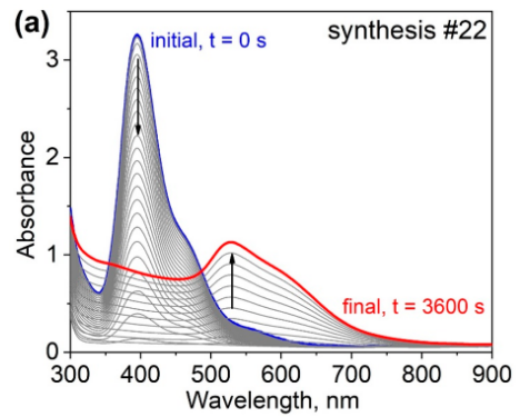
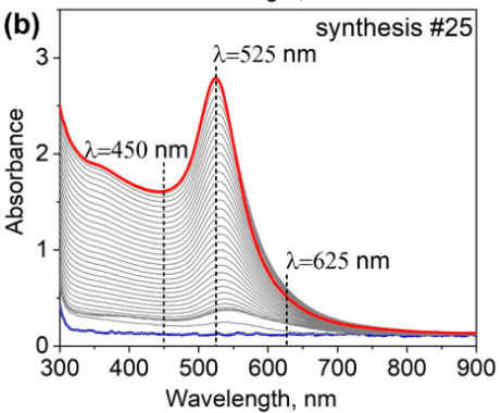
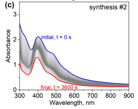
The UV/Vis spectra over time Figure 2 show the different stages.
Figure Figure 2 (a) shows the peak at 400 nm from the [AuBr₄]⁻ complex in blue. This peak disappears and a new peak grows at 525 nm, indicating the formation of gold nanoparticles. Figure Figure 2 (b) does not show the initial peak; the first stage goes very fast. It only shows the resultant peak at 525 nm, characteristic for spherical gold particles. Figure Figure 2 (c) shows the initial peak has not disappeared after 1 hour, indicating a slower reaction rate in this case.
3 groups
Figure Figure 3 shows the UV/Vis spectra of all 30 samples. The spectra can be grouped into three categories based on their behavior:
- Peak only at 400 nm, intial stage of [AuBr4]
- Peak only at 525, spherical gold nano particle
- Broadened peak at 525 and higher or multiple plateau with peaks at 525 and higher for longer nano particle
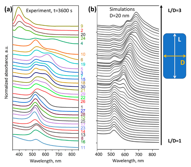
The peaks at 400 nm are not visible in the theoretical model. The model used here pashkovQuantitativeAnalysisUV2021 I discussed in a previous post. It deals with spherical and rod-shaped gold nano-particles; not with the formation process.
While some qualitative features are of the theoretical spectra are present, the experimental spectra are clearly different; representing the complex formation process of gold nanoparticles.
Machine learning
If the nanoparticles were formed during the synthesis, what was the shape of the nanoparticles and the time of their formation?
Machine learning was used to answer these questions, roughly:
- Did nano particles form during the 60 minutes?
- Were the nano particles spherical or elongated?
- Did it take more than 1500 s to form nano particles
The spectrum descriptors \(\chi_1\) and \(\chi_2\) were used in constructing labels for the machine learning model. These descriptors are defined in Table Table 1. So the spectrum forms the output space of the models.
The input of the models were the three synthesis parameters, linear combinations thereof and quadratic combinations; see table Table 1.
The classifiers are thus mapping synthesis parameters to spectral properties. The mapping learned.
| Descriptor | comment |
|---|---|
| Spectra | |
| \(\chi_1 = A(525)/A(450)\) | normalized height of the SPR maximum |
| \(\chi_2 = A(625)/A(525)\) | asymmetry of the SPR maximum |
| Synthesis | |
| Au, AA, CTAB | variable components in the synthesis |
| \(c_1 \cdot \text{Au} + c_2 \cdot \text{AA} + c_3 \cdot \text{CTAB}\); \(c_i = \pm 1\) | linear combinations of initial parameters |
| Au\(\cdot\)AA, Au\(\cdot\)CTAB, AA\(\cdot\)CTAB | products of the initial parameters |
| # | Target | Descriptor | Class 0 | Class 1 | Class 2 |
|---|---|---|---|---|---|
| 1 | Particle Formation | \(\chi_1 = \frac{A(525)}{A(450)}\) | \(\chi_1 < 1\) (none) |
\(1 < \chi_1 < 1.5\) (intermediate) |
\(\chi_1 > 1.5\) (significant) |
| 2 | Particle Shape | \(\chi_2 = \frac{A(625)}{A(525)}\) | \(\chi_1 < 1\) (no particles) |
\(\chi_2 < 0.7\) (spherical) |
\(\chi_2 > 0.7\) (elongated) |
| 3 | Formation Time | \(\tau\) when \(\chi_1 > 1\) | \(\tau > 4000\) s (late/none) |
\(1500 < \tau < 4000\) s (intermediate) |
\(\tau < 1500\) s (early) |
Feature selection
The extra tree model was used to perform feature selection in combination with leave-one-out cross validation.
Extra trees (Extremely randomized trees) is a tree ensemble method that is more robust than random forest and can be used with fewer data points.
| Target Variable | Selected Triple of Synthesis Descriptors | Classification Accuracy |
|---|---|---|
| χ₁ (particle formation) |
CTAB, Au, acid | 0.60 |
| CTAB, AA − CTAB·Au − AA | 0.69 | |
| AA − CTAB, Au·AA·Au − AA − CTAB | 0.79 | |
| χ₂ (particle shape) |
CTAB, Au, Acid | 0.57 |
| AA + CTAB, Au, Au·AA | 0.75 | |
| Au + AA + CTAB, Au − AA, Au − AA − CTAB | 0.79 | |
| τ (formation time) |
CTAB, Au, acid | 0.70 |
| CTAB, Au − AA + CTAB, Au − AA | 0.82 | |
| Au·AA, Au − AA + CTAB, Au − AA − CTAB | 0.83 |
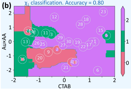
For \(\chi_1\) and \(\tau\) classifiers, the feature space could be reduced further to 2 descriptors. In figure Figure 4, the decision boundary of the 3 classes for \(\chi_1\) are visible.
Leave-One-Out Cross-Validation (LOOCV)
The leave one-out evaluation used here is prone to over-fitting.
The procedure consists of training on 29 points and testing on 1 point. This is repeated 30 times. With Extra Trees using 100 estimators on 29 training points, the model has high capacity relative to the data size
The authors had to repeat LOOCV 5 times and average results due to randomness in the Extra Trees algorithm. This suggests high variance in the performance estimates Individual LOOCV runs likely produced quite different accuracy values
Risk of Overfitting
The model could be learning patterns specific to these 30 experiments rather than general principles With such few data points, the model might memorize specific parameter combinations The 60-83% accuracy suggests it’s not completely overfitting (would be ~100%) but generalization is questionable; especially for those areas in 2D space with no training examples.
Even with Latin hypercube sampling, 30 points in a 3D parameter space provides sparse coverage The model’s ability to predict outcomes for parameter combinations far from the training data is uncertain
With only 30 points, the authors couldn’t afford a separate test set It’s the best they could do given the experimental constraints
High throughput experiment
The authors experiment with a miniaturized and automated version of the experiment that completed 60 experiments in just 2 hours.
This may be a good way to get started quickly with experimenting and developing machine learning along side. The authors note they there some issues with the miniature version.
For some combinations of flows, we have observed a plasmon peak shift toward lower wavelength, which was not observed in batch experiments. We attribute this shift to the formation of the AuAg alloy
As expected, some new effects are introduced. It is questionable how to extrapolate the results to a large scale production setup.
Lessons
With only 30 data points, the authors managed to distill some knowledge on gold nano particle synthesis. Some crucial parts are
- Limit to varying 3 production parameters
- Observe 3 groups of synthesis behaviour in the spectra
- Characterize the groups in terms of simple spectral quantities
- Simplify the spectrum prediction problem to a classification problem
- Use of robust learner like extra trees
- Feature selection
The paper positions this as a “proof of concept” for using ML with small synthesis datasets
The results should be viewed as demonstrating the feasibility of the ML approach rather than providing a robust, generalizable model. For production use, many more synthesis experiments would be needed.
It is also not clear how to extrapolate results to a production setting, to a different lab or different operator.